Cubic Spline Interpolation
Cubic spline interpolation is a mathematical method commonly used to construct new points within the boundaries of a set of known points. These new points are function values of an interpolation function (referred to as spline), which itself consists of multiple cubic piecewise polynomials. This article explains how the computation works mathematically.
After an introduction, it defines the properties of a cubic spline, then it lists different boundary conditions (including visualizations), and provides a sample calculation. Furthermore, it acts as a reference for the mathematical background of the cubic spline interpolation tool on tools.timodenk.com which is introduced at the end of the article.
Introduction
Cubic spline interpolation is the process of constructing a spline $f:[x_1,x_{n+1}]\rightarrow\mathbb{R}$ which consists of $n$ polynomials of degree three, referred to as $f_1$ to $f_n$. A spline is a function defined by piecewise polynomials. Opposed to regression, the interpolation function traverses all $n+1$ pre-defined points of a data set $\mathcal{D}$. The resulting function has the following structure:$$
f\left(x\right)=\begin{cases}
a_1x^3+b_1x^2+c_1x+d_1&\text{if }x\in\left[x_1,x_2\right]\\
a_2x^3+b_2x^2+c_2x+d_2&\text{if }x\in\left(x_2,x_3\right]\\
\dots\\
a_nx^3+b_nx^2+c_nx+d_n&\text{if }x\in\left(x_{n},x_{n+1}\right].
\end{cases}$$Note that all polynomials are just valid within an interval; they compose the interpolation function. While extrapolation predicts a development outside the range of the data, interpolation works just within the data boundaries $[x_1,x_{n+1}]$.
With properly chosen coefficients $a_i$, $b_i$, $c_i$, and $d_i$ for the polynomials, the resulting function traverses the points smoothly. For determining the coefficients, several equations are formulated which all together compose a uniquely solvable system of equations.

Table of Notation
| Symbol | Description |
|---|---|
| $\mathcal{D}$ | $n+1$ data points, a set of ordered pairs $\left(x,y\right)$ |
| $\left(x_i,y_i\right)$ | $i$th element in $\mathcal{D}$ under the condition $x_i\lt x_{i+1}$ (leftmost point: $\left(x_1,y_1\right)$) |
| $f:[x_1,x_{n+1}]\rightarrow\mathbb{R}$ | Interpolation function (spline) which predicts new points and consists of $n$ polynomials |
| $f_i:[x_i,x_{i+1}]\rightarrow\mathbb{R}$ | $i$th polynomial of third degree: $a_ix^3+b_ix^2+c_ix+d_i$ |
Properties of a Cubic Spline
In order to determine the $4n$ coefficients of all polynomials, several equations must be stated. First of all, every polynomial is known to pass through exactly two points. Therefore, the $2n$ equations $$
\begin{align}
f_1(x_1)&=y_1\\
f_1(x_2)&=y_2\\
f_2(x_2)&=y_2\\
f_2(x_3)&=y_3\\
\cdots\\
f_n(x_n)&=y_n\\
f_n(x_{n+1})&=y_{n+1},
\end{align}$$written-out as$$
\begin{align}
a_1x_1^3+b_1x_1^2+c_1x_1+d_1&=y_1\\
a_1x_2^3+b_1x_2^2+c_1x_2+d_1&=y_2\\
a_2x_2^3+b_2x_2^2+c_2x_2+d_2&=y_2\\
a_2x_3^3+b_2x_3^2+c_2x_3+d_2&=y_3\\
\dots\\
a_nx_n^3+b_nx_n^2+c_nx_n+d_n&=y_n\\
a_nx_{n+1}^3+b_nx_{n+1}^2+c_nx_{n+1}+d_n&=y_{n+1},
\end{align}
$$are applicable. They express that at $x=x_1$, the value of the first polynomial is equal to $y_1$, and at $x=x_2$, the value is $y_2$. For the point where the second polynomial begins ($x=x_2$), which is exactly where the first polynomial has ended, the second polynomial’s value is $y_2$. At $x=x_3$, it is $y_3$, and so forth.
Furthermore, the first and second derivative of all polynomials are identical in the points where they _touch _their adjacent polynomial. The derivatives of polynomials of degree three are $\frac{d}{dx}f_i\left(x\right)=3a_ix^2+2b_ix+c_i$ and $\frac{d^2}{dx^2}f_i\left(x\right)=6a_ix+2b_i$. $f_1$ touches the second polynomial $f_2$ at $x_2$, the second the third at $x_3$, and so forth until $f_{n-1}$ touches $f_n$ at $x_n$:$$
\begin{align}
\frac{d}{dx}f_1(x)&=\frac{d}{dx}f_2(x)&\vert_{x=x_2}\\
\frac{d}{dx}f_2(x)&=\frac{d}{dx}f_3(x)&\vert_{x=x_3}\\
\cdots\\
\frac{d}{dx}f_{n-1}(x)&=\frac{d}{dx}f_n(x)&\vert_{x=x_n}.
\end{align}
$$ Evaluated at the corresponding $x$ values, that gives
$$
\begin{align}
3a_1x_2^2+2b_1x_2+c_1&=3a_2x_2^2+2b_2x_2+c_2\\
3a_2x_3^2+2b_2x_3+c_2&=3a_3x_3^2+2b_3x_3+c_3\\
\dots\\
3a_{n-1}x_n^2+2b_{n-1}x_n+c_{n-1}&=3a_nx_n^2+2b_nx_n+c_n.
\end{align}
$$ Equivalently, for the second derivative, the same is done by stating$$
\begin{align}
\frac{d^2}{dx^2}f_1(x)&=\frac{d^2}{dx^2}f_2(x)&\vert_{x=x_2}\\
\frac{d^2}{dx^2}f_2(x)&=\frac{d^2}{dx^2}f_3(x)&\vert_{x=x_3}\\
\cdots\\
\frac{d^2}{dx^2}f_{n-1}(x)&=\frac{d^2}{dx^2}f_n(x)&\vert_{x=x_n},
\end{align}
$$ written-out as
$$
\begin{align}
6a_1x_2+2b_1&=6a_2x_2+2b_2\\
6a_2x_3+2b_2&=6a_3x_3+2b_3\\
\dots\\
6a_{n-1}x_n+2b_{n-1}&=6a_nx_n+2b_n.
\end{align}$$
This adds another $2\left(n-1\right)$ equations.
Boundary Conditions
In order to be able to solve the system of equations, two more pieces of information are required. Arbitrary constraints like setting the third derivative in the (say) fourth point to zero may be used. However, the selection of a boundary condition, consisting of a pair of equations, is the commonly used method. The four conditions “natural spline”, “not-a-knot spline”, “periodic spline”, and “quadratic spline”, are described in detail below.
Natural Spline
The natural spline is defined as setting the second derivative of the first and the last polynomial equal to zero in the interpolation function’s boundary points:
$$\begin{align}
6a_1x_1+2b_1&=0\\
6a_nx_{n+1}+2b_n&=0.\\
\end{align}$$The visual interpretation is that the function’s change of steepness approaches zero in the first and last point.

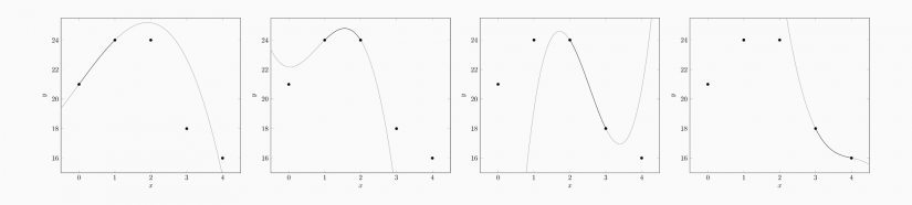
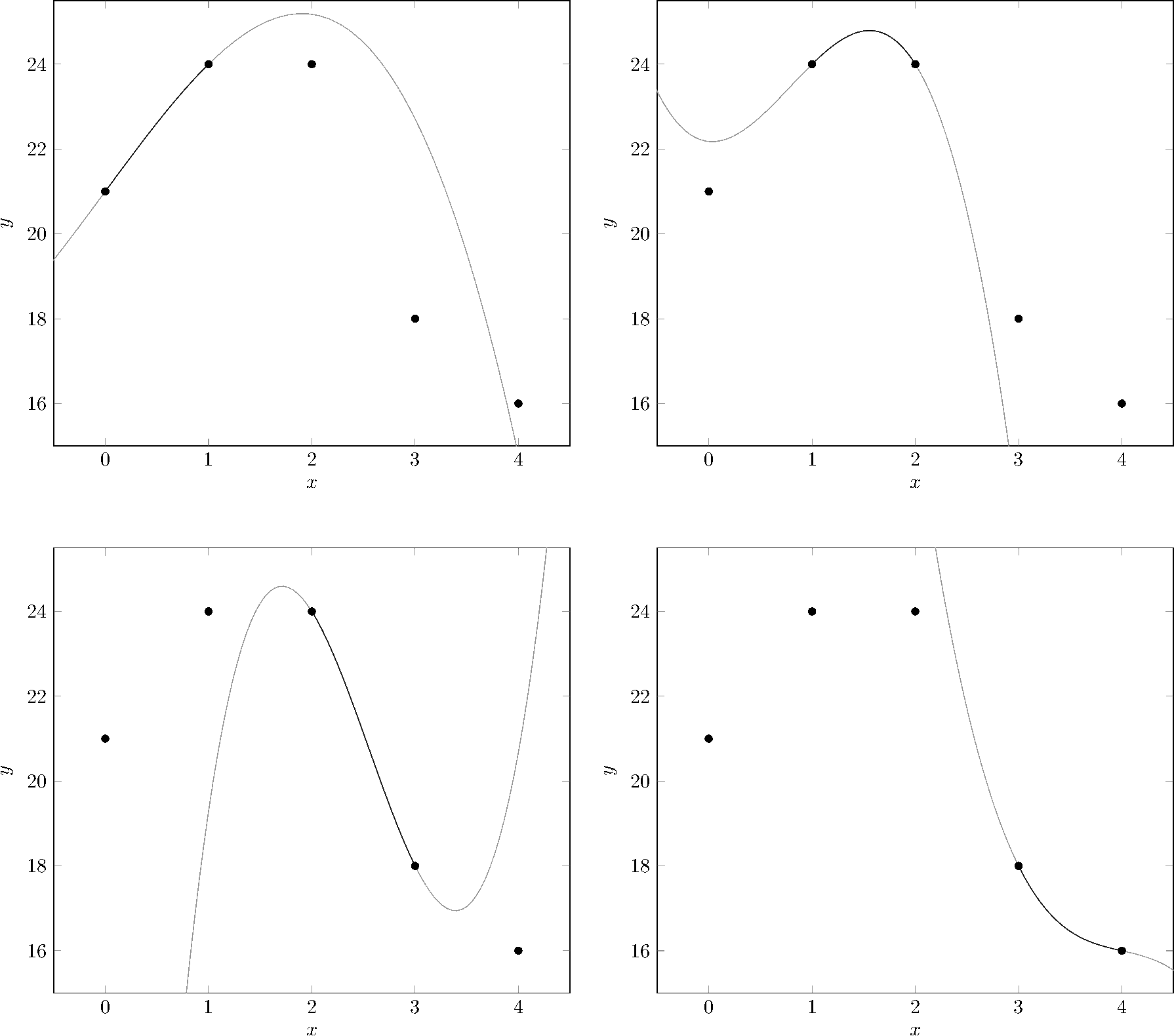
Not-a-Knot Spline
For the not-a-knot boundary condition, the first two polynomials’ third derivatives are equal in the point where they touch ($x_2$) each other. The same applies to the last two polynomials which touch at $x_n$, giving $$\begin{align}
\frac{d^3}{dx^3}f_1\left(x\right)&=\frac{d^3}{dx^3}f_2\left(x\right)&\vert_{x=x_2}\\
\frac{d^3}{dx^3}f_{n-1}\left(x\right)&=\frac{d^3}{dx^3}f_n\left(x\right)&\vert_{x=x_n}.
\end{align}$$
After calculating the derivatives this can be broken down to setting $$\begin{align}
a_1&=a_2\\
a_{n-1}&=a_n;
\end{align}$$that is making the $a$-coefficients equal to each other. The resulting plot can be seen in the following figure:

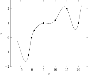
Periodic Spline
For a periodic interpolation, the last polynomial’s first and second derivative are set to be equal to the first polynomial’s first and second derivative. Graphically, this means that the function is tileable. This can be particularly helpful if $f(x_1)=f(x_{n+1})$, but works just as well with a function where the $y$ values of the first and last point differ. The figure below shows that $f_1$ can be copied and attached to the last point and the last polynomial $f_n$ to the first point, without making the function look odd.
The corresponding equations are
$$\begin{align}
3a_1x_1^2+2b_1x_1+c_1&=3a_nx_{n+1}^2+2b_nx_{n+1}+c_n\\
6a_1x_1+2b_1&=6a_nx_{n+1}+2b_n.\\
\end{align}$$
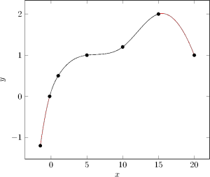
Quadratic Spline
The quadratic boundary condition defines the first and the last polynomial to be quadratic which makes this method the simplest one. The two parabolas are highlighted in red in the plot below. Mathematically spoken, the first coefficient of both polynomials is equal to zero: $a_1=a_n=0$.
Sample Calculation
This section performs a sample calculation with a real set of data and the “natural” boundary condition. Its purpose is to demonstrate how the equations are determined and actually turned into an interpolation function.
Given the set of points $$\mathcal{D}=\left\{\left(0,21\right),\left(1,24\right),\left(2,24\right),\left(3,18\right),\left(4,16\right)\right\},$$ the interpolation function will consist of $\left\lvert\mathcal{D}\right\rvert-1=4$ polynomials, namely $f_1$, $f_2$, $f_3$, and $f_4$. Each is of degree three: $f_i=a_ix^3+b_ix^2+c_ix+d_i$. The first polynomial $f_1$ is known to pass through the first and the second point, therefore $f_1\left(0\right)=21$ and $f_1\left(1\right)=24$. Equivalently, the second polynomial traverses the second and third point and so forth, leading to the equations
$$\begin{align}
f_2\left(1\right)&=24\\
f_2\left(2\right)&=24\\
f_3\left(2\right)&=24\\
f_3\left(3\right)&=18\\
f_4\left(3\right)&=18\\
f_4\left(4\right)&=16.
\end{align}$$
Furthermore, the first and second derivatives of all adjacent polynomials are equal in the point where they touch. The $f_1$ touches $f_2$ at $x=1$, leading to $$\begin{align}\frac{d}{dx}f_1(x)&=\frac{d}{dx}f_2(x)&\vert_{x=1},\end{align}$$ which is, after taking the derivative, equal to $$3a_1+2b_1+c_1=3a_2+2b_2+c_2.$$ Again, the same can be done for the other polynomials, giving $$\begin{align}
12a_2+8b_2+c_2&=12a_3+8b_3+c_3\\
27a_3+18b_3+c_3&=27a_4+18b_4+c_4.
\end{align}$$ The second derivative is handled in the same way so the following three equations apply:
$$\begin{align}
6a_1+2&=6a_2+2\\
12a_2+2&=12a_3+2\\
18a_3+2&=18a_4+2\\
\end{align}$$
The final two pieces of information are contained in the chosen boundary condition which in this example is the natural spline. The corresponding equations are
$$\begin{align}
2b_1&=0\\
24a_4+2b_4&=0.
\end{align}$$
All equations are forming a linear system of equations which can be written in matrix notation.
- Row 1 to 8: Equations expressing that the polynomials traverse the points in $\mathcal{D}$.
- Row 9 to 11: The first derivative of two adjacent polynomials is equal in the point where they touch.
- Row 12 to 14: The second derivative of two adjacent polynomials is equal in the point where they touch.
- Row 15 and 16: The boundary condition (natural spline).
$$
\begin{bmatrix}
0 & 0 & 0 & 1 & 0 & 0 & 0 & 0 & 0 & 0 & 0 & 0 & 0 & 0 & 0 & 0 \\
1 & 1 & 1 & 1 & 0 & 0 & 0 & 0 & 0 & 0 & 0 & 0 & 0 & 0 & 0 & 0 \\
0 & 0 & 0 & 0 & 1 & 1 & 1 & 1 & 0 & 0 & 0 & 0 & 0 & 0 & 0 & 0 \\
0 & 0 & 0 & 0 & 8 & 4 & 2 & 1 & 0 & 0 & 0 & 0 & 0 & 0 & 0 & 0 \\
0 & 0 & 0 & 0 & 0 & 0 & 0 & 0 & 8 & 4 & 2 & 1 & 0 & 0 & 0 & 0 \\
0 & 0 & 0 & 0 & 0 & 0 & 0 & 0 & 27 & 9 & 3 & 1 & 0 & 0 & 0 & 0 \\
0 & 0 & 0 & 0 & 0 & 0 & 0 & 0 & 0 & 0 & 0 & 0 & 27 & 9 & 3 & 1 \\
0 & 0 & 0 & 0 & 0 & 0 & 0 & 0 & 0 & 0 & 0 & 0 & 64 & 16 & 4 & 1 \\\hdashline
3 & 2 & 1 & 0 & -3 & -2 & -1 & 0 & 0 & 0 & 0 & 0 & 0 & 0 & 0 & 0 \\
0 & 0 & 0 & 0 & 12 & 4 & 1 & 0 & -12 & -4 & -1 & 0 & 0 & 0 & 0 & 0 \\
0 & 0 & 0 & 0 & 0 & 0 & 0 & 0 & 27 & 6 & 1 & 0 & -27 & -6 & -1 & 0 \\\hdashline
6 & 2 & 0 & 0 & -6 & -2 & 0 & 0 & 0 & 0 & 0 & 0 & 0 & 0 & 0 & 0 \\
0 & 0 & 0 & 0 & 12 & 2 & 0 & 0 & -12 & -2 & 0 & 0 & 0 & 0 & 0 & 0 \\
0 & 0 & 0 & 0 & 0 & 0 & 0 & 0 & 18 & 2 & 0 & 0 & -18 & -2 & 0 & 0 \\\hdashline
0 & 2 & 0 & 0 & 0 & 0 & 0 & 0 & 0 & 0 & 0 & 0 & 0 & 0 & 0 & 0 \\
0 & 0 & 0 & 0 & 0 & 0 & 0 & 0 & 0 & 0 & 0 & 0 & 24 & 2 & 0 & 0 \\
\end{bmatrix}
\begin{bmatrix}
a_1\\
b_1\\
c_1\\
d_1\\
a_2\\
b_2\\
c_2\\
d_2\\
a_3\\
b_3\\
c_3\\
d_3\\
a_4\\
b_4\\
c_4\\
d_4\\
\end{bmatrix}=\begin{bmatrix}
21\\24\\24\\24\\24\\18\\18\\16\\0\\0\\0\\0\\0\\0\\0\\0
\end{bmatrix}
$$
This system of equations can be solved (e.g. with Gaussian elimination) so that the function coefficients are calculated and the interpolation function
$$f(x) = \begin{cases}-0.30357 x^3 + 3.3036x + 21& \text{if } x \in [0,1]\\-1.4821x^3 + 3.5357x^2 -0.23214 x + 22.179& \text{if } x \in (1,2]\\3.2321x^3 -24.750x^2 + 56.339 x -15.536& \text{if } x \in (2,3]\\-1.4464x^3 + 17.357 x^2 -69.982 x + 110.79& \text{if } x \in (3,4].\end{cases}
$$can be written down. $f(x)$ is plotted in the figure below.

Online Tool
The cubic spline interpolation tool on tools.timodenk.com performs a cubic spline interpolation and visualizes the resulting function derived from a data set provided by the user. It offers selection of the boundary conditions and of the axes scaling. If needed, the corresponding $\LaTeX$ code for rendering the interpolation function in a document may be exported. The latter was also used to create the figures of this article. Through tools.timodenk.com, there is also access to linear, quadratic, and polynomial interpolation tools.
As a side note for developers, it is worth mentioning that a user of the tool reported a reproducible, weird interpolation result for a specific set of data. As it turned out, this was caused by the floating point precision of JavaScript which was too low for computing the coefficients from the system of equations without significant loss of precision. The issue was resolved by using the library Math.js. It features among other things a BigNumber class for very high precision numbers, which are now in use.