Least Squares Derivation

The least squares optimization problem searches for a vector, that minimizes the euclidean norm in the following statement as much as possible: $$x_\text{opt}=\arg\min_x\frac{1}{2}\left\lVert Ax-y\right\rVert^2_2,.$$This article explains how $x_\text{opt}=(A^\top A)^{-1}A^\top y$, the solution to the problem, can be derived and how it can be used for regression problems.

Derivation

In order to get a formula for $x_\text{opt}$, we start by expanding the euclidean norm. $\left\lVert v\right\rVert_2$ is defined as the square root of the sum of all squared vector elements. The root cancels out with the square which is contained in the problem definition and we are therefore left with the sum of all squared elements. That, however, is equal to the dot product $v\cdot v$ which in turn equals $v^\top v$. In the second line we expand the factor and, subsequently (in line 3), wrap all terms of the sum with the trace function. We can do so because each value passed to trace is a scalar and $\forall \gamma\in\mathbb{R}\left[\text{tr}\left(\begin{bmatrix}\gamma\end{bmatrix}\right)=\gamma\right]$ applies.
$$
\begin{align}
\frac{1}{2}\left\lVert Ax-y\right\rVert^2_2=&\frac{1}{2}\left(Ax-y\right)^\top \left(Ax-y\right)\\
=&\frac{1}{2}\left(x^\top A^\top Ax-y^\top Ax-x^\top A^\top y+y^\top y\right)\\
=&\frac{1}{2}\left(\text{tr}\left(x^\top A^\top Ax\right)-2\text{tr}\left(y^\top Ax\right)+\text{tr}\left(y^\top y\right)\right)
\end{align}
$$

The trace function makes differentiation easier, as we can apply the following two rules
$$
\begin{align}
\frac{\partial}{\partial X}\text{tr}\left(AXX^\top B\right)=&\left(A^\top B^\top +BA\right)X,,\\
\frac{\partial}{\partial X}\text{tr}\left(AXB\right)=&A^\top B^\top ,,\\
\end{align}
$$to the first and the second part of the sum respectively, when taking the partial derivatives with respect to the vector $x$. The third part of the sum is independent from $x$ and can therefore be dropped. $$
\begin{align}
\nabla_x\frac{1}{2}\left\lVert Ax-y\right\rVert^2_2=&\nabla_x\frac{1}{2}\left(\text{tr}\left(x^\top A^\top Ax\right)-2\text{tr}\left(y^\top Ax\right)+\text{tr}\left(y^\top y\right)\right)\\
=&\frac{1}{2}\nabla_x\left(\text{tr}\left(Axx^\top A^\top \right)-2\text{tr}\left(Axy^\top \right)\right)\\
=&\frac{1}{2}\left(2A^\top Ax-2A^\top y\right)\\
=&A^\top Ax-A^\top y,.
\end{align}
$$

Because we are searching for the lowest point, we set the derivative equal to zero. At this point the $x$ value is the optimal solution $x_\text{opt}$ to the original problem. With some equivalent transformations we isolate $x_\text{opt}$ and are left with the equation that we wanted to derive:
$$
\begin{align}
A^\top Ax_\text{opt}-A^\top y=&0\\
A^\top Ax_\text{opt}=&A^\top y\\
x_\text{opt}=&\left(A^\top A\right)^{-1}A^\top y
\end{align}
$$

Regression

In regression, least squares is used to determine the adjustable parameters of a model function. The set of data points $\mathcal{D}$ contains $n$ tuples $\left(x_i,y_i\right)$. The variable that was previously called $x$ is a vector of unknown function variables named $a_\mathcal{D}$. For the quadratic model function $f(x)=a_2x^2+a_1x+a_0$ the vector would be $a_\mathcal{D}=\begin{bmatrix}a_2&a_1&a_0\end{bmatrix}^\top $ (the order is arbitrary). The matrix $A_\mathcal{D}$ holds the factors that each adjustable model function parameter has if a given tuple is plugged into the function. Note that the column order must match the order of the elements in $a_\mathcal{D}$. $y_\mathcal{D}=\begin{bmatrix}y_1 & \cdots & y_n\end{bmatrix}^\top $ is a vector, containing all $y$-values of $\mathcal{D}$. Opposed to interpolation, the problem is overdetermined and the resulting regression function will therefore not traverse all data points.

The resulting statement
$$\arg\min_{a_\mathcal{D}}\frac{1}{2}\left\lVert\begin{bmatrix}x_1^2 & x_1 & 1\\\vdots & \vdots & \vdots \\x_n^2 & x_n & 1\end{bmatrix}\begin{bmatrix}a_2\\a_1\\a_0\end{bmatrix}-\begin{bmatrix}y_1 \\ \vdots \\ y_n\end{bmatrix}\right\rVert^2_2$$ can be intuitively thought of as the search for the function variables $a$ for which the function evaluation is as close as possible to the desired outputs $y$. Measure for closeness is the euclidean distance. Note that all values are known except for $a_2$, $a_1$, and $a_0$.

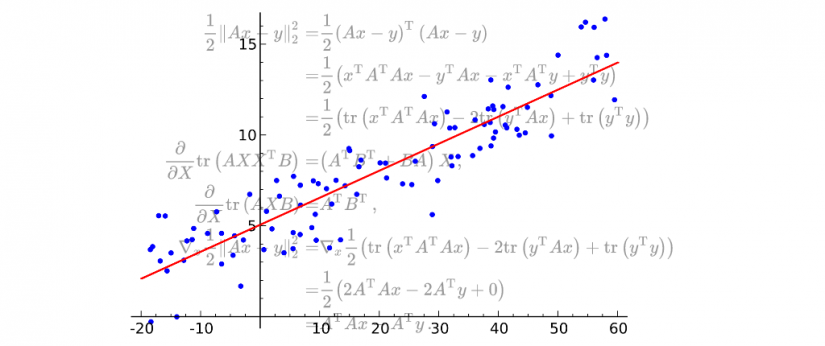
MATLAB Sample Calculation

Given a set of points, underlying a linear function $y(x)=a_1x+a_0$, the variables $A$ and $y$ are initialized in MATLAB with the following snippet.

y = randn(100,1)  % random y values
n = numel(y)  % number of points
x = 1/n * 10 * [1:n]'  % x values
y = y + x  % add slope to y values
A = [x ones(n,1)]  % compose A matrix
plot(x,y)

The actual parameter calculation according to $\left(A^\top A\right)^{-1}A^\top y$ works as follows.

a = inv(transpose(A)*A)*transpose(A)*y

It yields for example $a_1=1.0225$ and $a_2=0.0012$ resulting in the regression function $f(x)=1.0225x+0.0012$.