[Paper Recap] Multiple Hypotheses Prediction
The paper Learning in an Uncertain World: Representing Ambiguity Through Multiple Hypotheses was publish by Christian Rupprecht et al. in late 2016. The authors propose a training technique for machine learning models which makes them predict multiple distinct hypotheses. This is an advantage for many prediction tasks, in which uncertainty is part of the problem. In this article I am going to summarize the paper and name further thoughts.
Introduction
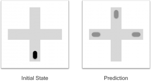
Rupprecht et al. open their introduction by giving examples of tasks that are dealing with uncertainty. An illustrative example is a car that drives towards an intersection (at $t=0$). It has three options, namely turning left, driving straight, or turning right. A model is trained to process an image taken at $t=0$ and output an image that shows the scene’s state at $t=1$ (that is after the car has made its way beyond the intersection). Each of these three options has a probability of one third. A Single Hypothesis Prediction (SHP) model, which can be described by a function $f_\theta:\mathcal{X}\rightarrow\mathcal{Y}$, would output a mixture of all three options, as illustrated in the following figure. $\mathcal{X}$ and $\mathcal{Y}$ denote the set of possible inputs and outputs, respectively.
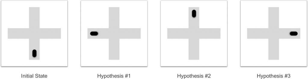
A Multiple Hypotheses Prediction (MHP) model, however, is capable of making $M$ predictions. $M$ is a hand-tuned hyper parameter of MHP models. An ideal outcome, with $M=3$, is shown in the figure below. The function signature changes to $f_\theta:\mathcal{X}\rightarrow\mathcal{Y}^M,.$
In the related work section, the authors name among others (1) mixture density networks (MDNs), (2) multiple choice learning which is closely related to their work, and (3) CNN training with soft probabilistic class assignments, Gao et al. [1].
Multiple Hypotheses Prediction Models
An MHP model can be interpreted as a vector of generators which typically, but not necessarily, share some of their weights $\theta$. Further details on how to convert an SHP model into an MHP model will follow later. The principles of the training techniques that Rupprecht et al. use in their paper (see Equation 6) were proposed by Guzman-Rivera et al. [2] and later used, e.g. by Lee et al. [3]. They are to minimize $$\int_\mathcal{X}\sum_{j=1}^M\int_\mathcal{Y_j(x)}\mathcal{L}\left(f_{\theta,j}(x),y)p(x)p(y\mid x)\right)dy\ dx,,$$ where $\mathcal{L}$ denotes an arbitrary loss function and $p(x)p(y\mid x)$ weights the importance of each sample depending on its commonness. For each input $x$, the output set $\mathcal{Y}$ is split into $M$ parts, $\mathcal{Y}_1$ to $\mathcal{Y}_M$. This split corresponds to a Voronoi tesselation where the measure of distance is the loss function $\mathcal{L}$ and the cell’s center points are the $M$ generator outputs. Intuitively, the equation can be understood as follows: For each input $x\in\mathcal{X}$, iterate over every output $y\in\mathcal{Y}$ and sum up the weighted loss $\mathcal{L}$ with respect to the closest generator $f_{\theta,j}$. The key is, that bad generators which are far off will not be punished for that, because the generator weights are only being updated with the gradient $$\frac{\partial}{\partial\theta}\frac{1}{\lvert\mathcal{Y}_j\rvert}\sum_{y_i\in\mathcal{Y}_j}\mathcal{L}\left(f_{\theta,j}(x_i),y_i\right),,$$ induced solely by training samples $(x_i,y_i)$ within their own Voronoi cell $\mathcal{Y}_j$. Therefore multiple hypotheses can coexist.
Rupprecht et al. have noticed that updating only the closest generator can lead to a state where all but one generator are idle, due to the random weight initialization and the therefrom resulting random initial positioning. They tackle the problem by (1) employing a prediction drop out, which “introduces some [1%] randomness in the selection of the best hypothesis”, and (2) introducing a hyper parameter $\varepsilon$ called association relaxation. The idea is (see Equation 12 of the paper) to relax the learning rate: It is multiplied by $\frac{\varepsilon}{M-1}$ for every generator except for the best, where $1-\varepsilon$ is chosen. That way inactive generators will slowly move towards an area where they can take over more densely populated areas of the output space. However, this becomes less important over the course of training time, as most generators will have specialized eventually in certain areas of the output space. Therefore, I would suggest to apply an association relaxation decay, which gradually lowers $\varepsilon$ during training. The decay rate could be based on (a) the number of training epochs or, more sophisticated, (b) the burden sharing between the generators. The lower the number of idle generators, the lower should $\varepsilon$ be until it converges towards $0$.
There are multiple ways of setting up an MHP model, capable of predicting $M$ hypotheses:
- Duplicating an SHP model $M$ times. This is straightforward and increases the number of parameters significantly which reminds of Mixture-of-Expert layers [4]. Generators are not sharing their weights and must be initialized differently.
- Duplicating the last layer of an SHP model $M$ times (initialized with different weights). Each of the $M$ output layers is connected to the previous, shared layer in the same way, except the weights are different and trained individually. For this case, the authors state that “the number of predictions $M$ on training time is usually negligible” which is a big advantage. Furthermore, “information exchange between predictions” is possible.
- Branching at any given hidden layer and duplicating all following layers (with different weights). Generalization of the previous bullet point.
The authors have conducted several experiments to validate the technique: (1) A basic 2D example that gives an intuition for the Voronoi cells, (2) human pose estimation, (3) future frame prediction (high dimensional problem), and (4) multi-label image classification and segmentation. I found particularly relevant that the model has proven to produce sharper outputs than SHP models, when predicting future frames. This corresponds to the intuition that traditional SHP models undesirably average over possible outcomes.
Conclusion
The approach of generating multiple hypotheses is very natural and corresponds to many real world problems. In my opinion, the proposed method is very applicable not only because the number of weights remains low but also because of its generality and simplicity: Training comes only with the augmentation of measuring the distance to every hypothesis and updating the generator that was the closest.
The proposed MHP models do not deliver their hypotheses with likelihood (aka. confidence) information. For some real world applications, however, this measure is crucial as hypotheses can be completely beside it for some inputs. It was not part of the paper to discuss or develop such an attention-like mechanism.
References
- B.-B. Gao, C. Xing, C.-W. Xie, J. Wu, and X. Geng. Deep label distribution learning with label ambiguity. 2016.
- A. Guzman-Rivera, D. Batra, and P. Kohli. Multiple Choice Learning: Learning to Produce Multiple Structured Outputs. In Advances in Neural Information Processing Systems, 2012.
- S. Lee, S. P. S. Prakash, M. Cogswell, V. Ranjan, D. Crandall, and D. Batra. Stochastic multiple choice learning for training diverse deep ensembles. In Advances in Neural Information Processing Systems, pages 2119–2127, 2016.
- N. Shazeer, A. Mirhoseini, K. Maziarz, A. Davis, Q. Le, G. Hinton, J. Dean. Outrageously Large Neural Networks: The Sparsely-Gated Mixture-of-Experts Layer. 2017.